Lesson 2: First R Steps
The R command prompt is >. Again, it will be shown here, but you don’t type
it. It is just there in your R window to let you know R is inviting you
to submit a command. (If you are using RStudio, you’ll see it in the
Console pane.)
So, just type 1+1 then hit Enter. Sure enough, it prints out 2 (you
were expecting maybe 12108?):
> 1 + 1
[1] 2
But what is that [1] here? It’s just a row label. We’ll go into that
later, not needed quite yet.
Example: Nile River data
R includes a number of built-in datasets, mainly for illustration
purposes. One of them is Nile, 100 years of annual flow data on the
Nile River.
Let’s find the mean flow:
> mean(Nile)
[1] 919.35
Here mean is an example of an R function, and in this case Nile is
an argument — fancy way of saying “input” — to that function. That
output, 919.35, is called the return value or simply value. The act
of running the function is termed calling the function.
Another point to note is that we didn’t need to call R’s print
function. We could have typed,
> print(mean(Nile))Function calls in R (and other languages) work “from the inside out.” Here we are asking R to find the mean of the Nile data, then print the result.
But whenever we are at the R > prompt, any expression we type will be
printed out anyway, so there is no need to call print.
Since there are only 100 data points here, it’s not unwieldy to print
them out. Again, all we have to do is type Nile, no need to call
print:
> Nile
Time Series:
Start = 1871
End = 1970
Frequency = 1
  [1] 1120 1160  963 1210 1160 1160  813 1230 1370 1140  995  935 1110  994 1020
 [16]  960 1180  799  958 1140 1100 1210 1150 1250 1260 1220 1030 1100  774  840
 [31]  874  694  940  833  701  916  692 1020 1050  969  831  726  456  824  702
 [46] 1120 1100  832  764  821  768  845  864  862  698  845  744  796 1040  759
 [61]  781  865  845  944  984  897  822 1010  771  676  649  846  812  742  801
 [76] 1040  860  874  848  890  744  749  838 1050  918  986  797  923  975  815
 [91] 1020  906  901 1170  912  746  919  718  714  740
Now you can see how the row labels work. There are 15 numbers per row
here, so the second row starts with the 16th, indicated by [16]. The
third row starts with the 31st output number, hence the [31] and so
on.
Note that a set of numbers such as Nile is called a vector.
A first graph
R has great graphics, not only in base R but also in wonderful
user-contributed packages, such as ggplot2 and lattice. But
we’ll stick with base-R graphics for now, and save the more powerful yet
more complex ggplot2 for a later lesson.
We’ll start with a very simple, non-dazzling one, a no-frills histogram:
> hist(Nile)No return value for the hist function (there is one, but it is
seldom used, and we won’t go into it here), but it does create the
graph.
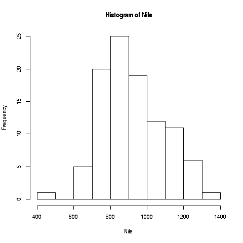
Your Turn: The
histfunction draws 10 bins for this dataset in the histogram by default, but you can choose other values, by specifying an optional second argument to the function, namedbreaks. E.g.> hist(Nile,breaks=20)would draw the histogram with 20 bins. Try plotting using several different large and small values of the number of bins.
Note: The
histfunction, as with many R functions, has many different options, specifiable via various arguments. For now, we’ll just keep things simple, and resist the temptation to explore them all.
R has lots of online help, which you can access via ?. E.g. typing
> ?histwill tell you to full story on all the options available for the hist function. Again, there are far too many for you to digest for now (most users don’t ever find a need for the more esoteric ones), but it’s a vital resource to know.
Your Turn: Look at the online help for
meanandNile.