Lesson 22: Linear Regression Analysis, I
Looking at the picture in the last lesson, it seems we could draw a straight line through that cloud of points that fits the points pretty well. Here is where linear regression analysis comes in.
We of course cannot go into the details of statistical methodology here, but it will be helpful to at least get a good definition set:
As mentioned, we treat the data as a sample from the (conceptual) population of all players, past, present and future. Accordingly, there is a population mean weight for each age group. It is assumed that those population means, when plotted against age, lie on some straight line.
In other words, our model is
mean weight = β0 + β1 height
where β0 and β1 are the intercept and slope of the population regression line.
So, we need to use the data to estimate the slope and intercept of that
straight line, which R’s lm (“linear model”) function does for us.
We’ll use the original dataset, since the one with rounded ages was just
to guide our intuition.
> lm(Weight ~ Age,data=mlb)

Call:
lm(formula = Weight ~ Age, data = mlb)

Coefficients:
(Intercept)          Age
   181.4366       0.6936
Here the call instructed R to estimate the regression line of weight
against age, based on the mlb data.
So the estimated slope and intercept are 0.6936 and 181.4366, respectively. (Remember, these are just sample estimates. We don’t know the population values.) R has a provision by which we can draw the line, superimposed on our scatter plot:
> abline(181.4366,0.6936)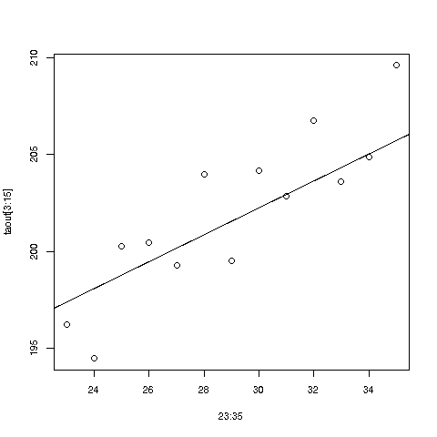
Your Turn: In the
mtcarsdata, fit a linear model of the regression of MPG against weight; what is the estimated effect of 100 pounds of extra weight?